Joint constraints

In practice, there are two main ways of modeling joints:

Reduced-coordinates approach.
Constraints-based approach.

Reduced-coordinates approach

The reduced-coordinates approach encodes the reduction of DOF directly into the equations of motion. For example, a 3D rigid-body attached to the ground with a revolute joint will have its position encoded by only one variable: the rotation angle. Therefore, integrating its motion only changes this one variable and doesn't need additional forces or mathematical constraints to be generated. The clear advantage is that there is no way for the physics engine to apply any motion other than that single rotation to this body, meaning there is no way the body shifts to a position that is not realistic, even if the dynamics solver does not converge completely.

Rapier implements this approach through MultibodyJointSet, where each joint is attached to its relevant rigid-bodies identified by their handle. The bevy_rapier plugin implements this approach through the MultibodyJoint component, where each joint is attached to its relevant rigid-bodies identified by their entity. Rapier implements this approach through MultibodyJointSet, where each joint is attached to its relevant rigid-bodies identified by their handle.

Rapier implements this approach through the multibody joints inserted with r3InsertMultibodyJoint, where each joint is attached to its relevant rigid-bodies identified by their handle.

Rapier implements this approach through the MultibodyJointSet (given by PhysicsWorld.multibody_joints), where each joint is attached to its relevant rigid-bodies identified by their handle.

Constraints-based approach

The constraints-based approach (or full-coordinates approach) is the most commonly available approach on other physics engines for video-games and animations. Here, a 3D rigid-body attached to the ground with a revolute joint will still have its position encoded by 6 variables (3 for translations and 3 for rotations) just like any rigid-body without a joint. Then the integrator will add mathematical constraints to the dynamic system to ensure forces are applied to simulate the reduction of the number of DOF as imposed by the joints. In practice, this means that the rigid-body will break the joint constraint if the constraint solver does not converge completely.

Rapier implements this approach through ImpulseJointSet, where each joint is attached to two distinct rigid-bodies identified by their rigid-body handles. The bevy_rapier plugin implements this approach through the ImpulseJoint component, where each joint is attached to two distinct rigid-bodies identified by their entities. Rapier implements this approach through ImpulseJointSet, where each joint is attached to two distinct rigid-bodies identified by their rigid-body handles.

Rapier implements this approach through the impulse joints inserted with r3InsertImpulseJoint, where each joint is attached to two distinct rigid-bodies identified by their rigid-body handles.

Rapier implements this approach through the ImpulseJointSet (given by PhysicsWorld.impulse_joints), where each joint is attached to two distinct rigid-bodies identified by their rigid-body handles.

More generally, the reduced-coordinates approach favors accuracy while the constraints-based approach favors versatility.

The following table compares the advantages and limitations of both approaches:

Reduced-coordinates approach	Constraints-based approach
Joints cannot be violated at all.	Joints can be violated if the solver does not converge.
Moderately large time-steps are possible.	Moderately large time-steps may make the simulation explode.
Large assemblies are stable.	Large assemblies easily break without a large number of solver iterations.
Adding/removing a joint is slow.	Adding/removing a joint is fast.
Joint forces are never computed explicitly, thus cannot be retrieved.	Joint forces are always computed and can be retrieved.
Topological restriction: bodies must be linked following a tree structure.	The link between bodies can form any graph.

The following schematics illustrate a configuration that can be simulated by a multibody (left assembly with a tree structure), and one that cannot (right assembly with a graph structure). The assembly on the left models a SCARA robotic arm with 3 rotational DOF (due to three revolute joints) and 1 translational DOF (due to one prismatic joint). The assembly on the right models a necklace with five pearls. It has a total of 15 rotational DOF (due to five ball joints):

Tree-like assembly

"Which approach should I use?"

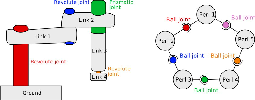
The choice of approach depends on the application. For robotics, the reduced-coordinates approach is generally preferred because of its accuracy and ease of use, e.g., for control, inverse kinematics, etc.

Video games traditionally favor the constraints-based approach since most existing physics libraries implement only this. Moreover if joint assemblies are small, and joints are frequently added and removed, the constraints-based approach will be more efficient. Some other physics libraries implement the reduced-coordinates approach as well but often using the Featherstone algorithm which is extremely unstable in practice.

Simulating closed loops like for a necklace cannot be achieved with the reduced-coordinates approach only. However, it is possible to combine both approaches by using joint constraints only to close the loops. Refer to the last section for details.

Multibodies

Multibodies implement the reduced-coordinates approach. A multibody is a set of multibody links attached together by a multibody joint.

Creating a multibody

The API to create a Multibody joint is similar to creating an Impulse Joint, refer to Joints, but insert those into the physics world with PhysicsWorld::insert_multibody_joint (instead of PhysicsWorld::insert_impulse_joint). Note that it returns None if the joint would make the multibody invalid, i.e., if both rigid-bodies are already part of the same multibody (which would create a loop), or if the second rigid-body is already attached to a parent link.

See Rapier's example for a demonstration of both approaches.

The API to create a multibody joint is similar to creating an impulse joint, refer to Joints, but add a MultibodyJoint component instead of an ImpulseJoint component. The root of the multibody is the rigid-body that isn't attached to any parent by a multibody joint:

Example 2D
Example 3D

/* Build a chain of three links attached with multibody joints. */
let mut parent = commands.spawn(RigidBody::Fixed).id();
for i in 1..=3 {
    let joint = RevoluteJointBuilder::new().local_anchor2(Vec2::new(0.0, 2.0));
    parent = commands
        .spawn((
            RigidBody::Dynamic,
            Collider::cuboid(0.5, 0.5),
            Transform::from_xyz(0.0, -2.0 * i as f32, 0.0),
            MultibodyJoint::new(parent, joint),
        ))
        .id();
}

/* Build a chain of three links attached with multibody joints. */
let mut parent = commands.spawn(RigidBody::Fixed).id();
for i in 1..=3 {
    let joint = RevoluteJointBuilder::new(Vec3::Z).local_anchor2(Vec3::new(0.0, 2.0, 0.0));
    parent = commands
        .spawn((
            RigidBody::Dynamic,
            Collider::cuboid(0.5, 0.5, 0.5),
            Transform::from_xyz(0.0, -2.0 * i as f32, 0.0),
            MultibodyJoint::new(parent, joint),
        ))
        .id();
}

After each simulation step, the coordinates and velocities of a multibody joint are written back into its MultibodyJointState component (automatically added alongside the MultibodyJoint). Modifying MultibodyJoint::parent re-attaches the joint to another rigid-body. Unlike impulse joints, multibody joints cannot be disabled.

See bevy_rapier's example for a demonstration of both approaches.

The API to create a Multibody joint is similar to creating an Impulse Joint, refer to Joints, but insert those into the physics world with World.createMultibodyJoint (instead of World.createImpulseJoint).

See Rapier's example for a demonstration of both approaches.

The API to create a multibody joint is similar to creating an impulse joint, refer to Joints, but insert those into the world with r3InsertMultibodyJoint (instead of r3InsertImpulseJoint). The root of the multibody is the rigid-body that isn't attached to any parent by a multibody joint. Note that the insertion fails (returning R3_INVALID_MULTIBODY_JOINT_HANDLE and reporting an R3_INVALID_ARGUMENT error) if the joint would make the multibody invalid, i.e., if both rigid-bodies are already part of the same multibody (which would create a loop), or if the second rigid-body is already attached to a parent link:

Example 2D
Example 3D

// The root of the multibody: a fixed rigid-body.
R2RigidBodyDesc root_desc = r2FixedRigidBodyDesc();
R2RigidBodyHandle root = r2InsertRigidBody(world, &root_desc);
// Three links, each attached to the previous one by a revolute multibody joint.
R2RigidBodyHandle parent = root;
R2MultibodyJointHandle last_joint = R2_INVALID_MULTIBODY_JOINT_HANDLE;
for (int i = 1; i <= 3; i++) {
    R2RigidBodyHandle link = insert_ball(world, r2Vector(2.0 * i, 0.0));
    R2JointDesc joint = r2RevoluteJointDesc();
    joint.localFrame2.translation = r2Vector(-2.0, 0.0);
    last_joint = r2InsertMultibodyJoint(parent, link, &joint);
    parent = link;
}

// The root of the multibody: a fixed rigid-body.
R3RigidBodyDesc root_desc = r3FixedRigidBodyDesc();
R3RigidBodyHandle root = r3InsertRigidBody(world, &root_desc);
// Three links, each attached to the previous one by a revolute multibody joint.
R3RigidBodyHandle parent = root;
R3MultibodyJointHandle last_joint = R3_INVALID_MULTIBODY_JOINT_HANDLE;
for (int i = 1; i <= 3; i++) {
    R3RigidBodyHandle link = insert_ball(world, r3Vector(0.0, 0.0, -2.0 * i));
    R3JointDesc joint = r3RevoluteJointDesc(r3Vector(1.0, 0.0, 0.0));
    joint.localFrame2.translation = r3Vector(0.0, 0.0, 2.0);
    last_joint = r3InsertMultibodyJoint(parent, link, &joint);
    parent = link;
}

A multibody joint is removed with r3RemoveMultibodyJoint. Its configuration can be read with r3MultibodyJoint_Desc, and replaced with r3MultibodyJoint_SetDesc (which reports an R3_INVALID_ARGUMENT error if the locked axes of the joint change, since they define the degrees of freedom of the multibody). The rigid-bodies attached by a multibody joint, i.e., its parent link then its own link, are given by r3MultibodyJoint_Bodies:

Example 2D
Example 3D

// Change the motor of an existing multibody joint.
R2JointDesc desc = r2MultibodyJoint_Desc(last_joint);
r2JointDesc_SetMotorVelocity(&desc, R2_AXIS_ANG_X, 1.0, 0.5);
r2MultibodyJoint_SetDesc(last_joint, &desc, 1);
// The rigid-bodies attached by the joint: its parent link, then its own link.
R2JointBodies bodies = r2MultibodyJoint_Bodies(last_joint);

// Change the motor of an existing multibody joint.
R3JointDesc desc = r3MultibodyJoint_Desc(last_joint);
r3JointDesc_SetMotorVelocity(&desc, R3_AXIS_ANG_X, 1.0, 0.5);
r3MultibodyJoint_SetDesc(last_joint, &desc, 1);
// The rigid-bodies attached by the joint: its parent link, then its own link.
R3JointBodies bodies = r3MultibodyJoint_Bodies(last_joint);

See the C testbed example for a demonstration of both approaches.

Generalized coordinates

The state of a multibody is described by its generalized coordinates (one per DOF of each of its joints) instead of the poses of its links. Its generalized velocities, i.e., the relative velocities along the free DOF of each of its joints, can be read with r3MultibodyJoint_GeneralizedVelocity and replaced with r3MultibodyJoint_SetGeneralizedVelocity. These functions apply to the whole multibody the given joint belongs to: their arrays have one element per DOF of the multibody, as given by r3MultibodyJoint_Ndofs. Note that the root of a multibody counts as a free link (with 6 DOF in 3D, and 3 DOF in 2D) if its rigid-body is dynamic:

Example 2D
Example 3D

// The number of degrees of freedom of the whole multibody (3 revolute joints: 3 DOF).
size_t ndofs = r2MultibodyJoint_Ndofs(last_joint);
R2Real *velocities = malloc(ndofs * sizeof(R2Real));
// Read the generalized velocities of the multibody, i.e., the relative angular velocity of each joint.
r2MultibodyJoint_GeneralizedVelocity(last_joint, velocities, ndofs);
// Stop every joint of the multibody.
for (size_t i = 0; i < ndofs; i++) {
    velocities[i] = 0.0;
}
r2MultibodyJoint_SetGeneralizedVelocity(last_joint, velocities, ndofs);
free(velocities);

// The number of degrees of freedom of the whole multibody (3 revolute joints: 3 DOF).
size_t ndofs = r3MultibodyJoint_Ndofs(last_joint);
R3Real *velocities = malloc(ndofs * sizeof(R3Real));
// Read the generalized velocities of the multibody, i.e., the relative angular velocity of each joint.
r3MultibodyJoint_GeneralizedVelocity(last_joint, velocities, ndofs);
// Stop every joint of the multibody.
for (size_t i = 0; i < ndofs; i++) {
    velocities[i] = 0.0;
}
r3MultibodyJoint_SetGeneralizedVelocity(last_joint, velocities, ndofs);
free(velocities);

warning

The multibody is only updated by the next simulation step after a multibody joint is inserted or removed. In particular, until that step, a root that isn't dynamic still counts as a free link in the DOF of the multibody.

Inverse kinematics

Multibodies support inverse kinematics: r3MultibodyJoint_InverseKinematics computes the displacements of the generalized coordinates of the multibody that move the link attached by the given joint toward a target pose. These displacements are then applied with r3MultibodyJoint_ApplyDisplacements. The R3InverseKinematicsOptions (initialized by r3DefaultInverseKinematicsOptions) select the axes of the target pose to reach (constrained_axes, one bit per axis like the lockedAxes of a joint), the maximum number of iterations of the solver, its damping, and its tolerances. An optional callback (given with its user data) lets you select the links that are allowed to move:

Example 2D
Example 3D

// Only try to reach the target translation, whatever the orientation of the last link.
R2InverseKinematicsOptions options = r2DefaultInverseKinematicsOptions();
options.constrained_axes = (1 << R2_AXIS_LIN_X) | (1 << R2_AXIS_LIN_Y);
R2Pose target = r2TranslationPose(r2Vector(0.5, 1.5));

// The displacements must be zero-initialized, with one entry per degree of freedom of the multibody.
size_t ndofs = r2MultibodyJoint_Ndofs(end_effector);
R2Real *displacements = calloc(ndofs, sizeof(R2Real));
// Compute the displacements moving the link of `end_effector` toward the target, then apply them.
r2MultibodyJoint_InverseKinematics(end_effector, &options, target, NULL, NULL, displacements, ndofs);
r2MultibodyJoint_ApplyDisplacements(end_effector, displacements, ndofs);
free(displacements);

// Only try to reach the target translation, whatever the orientation of the last link.
R3InverseKinematicsOptions options = r3DefaultInverseKinematicsOptions();
options.constrained_axes = (1 << R3_AXIS_LIN_X) | (1 << R3_AXIS_LIN_Y) | (1 << R3_AXIS_LIN_Z);
R3Pose target = r3TranslationPose(r3Vector(0.5, 1.5, 0.0));

// The displacements must be zero-initialized, with one entry per degree of freedom of the multibody.
size_t ndofs = r3MultibodyJoint_Ndofs(end_effector);
R3Real *displacements = calloc(ndofs, sizeof(R3Real));
// Compute the displacements moving the link of `end_effector` toward the target, then apply them.
r3MultibodyJoint_InverseKinematics(end_effector, &options, target, NULL, NULL, displacements, ndofs);
r3MultibodyJoint_ApplyDisplacements(end_effector, displacements, ndofs);
free(displacements);

The API to create a multibody joint is similar to creating an impulse joint, refer to Joints, but insert those into the world with world.multibody_joints.insert (instead of world.impulse_joints.insert). The root of the multibody is the rigid-body that isn't attached to any parent by a multibody joint. Note that the insertion returns None if the joint would make the multibody invalid, i.e., if both rigid-bodies are already part of the same multibody (which would create a loop), or if the second rigid-body is already attached to a parent link:

# The root of the multibody: a fixed rigid-body.
root = world.add_body(rp.RigidBody.fixed())
# Three links, each attached to the previous one by a revolute multibody joint.
parent = root
for i in range(1, 4):
    link = world.add_body(
        rp.RigidBody.dynamic(translation=(0.0, 0.0, -2.0 * i)),
        colliders=[rp.Collider.ball(0.5)],
    )
    joint = rp.RevoluteJoint.builder(axis=(1.0, 0.0, 0.0)).local_anchor2((0.0, 0.0, 2.0))
    # `insert` returns None if the joint would make the multibody invalid.
    last_joint = world.multibody_joints.insert(parent, link, joint)
    parent = link

A multibody joint can also be inserted with world.multibody_joints.insert_kinematic: the joint is then kinematic, i.e., its coordinates are entirely controlled by the application (e.g., through inverse kinematics) instead of being simulated. A multibody joint is removed with world.multibody_joints.remove. After its insertion, it is accessed with world.multibody_joints[handle], which returns a MultibodyJoint: a live view of the joint whose data property is its GenericJoint (exactly like ImpulseJoint.data): modifying it wakes up its rigid-bodies at the next simulation step. It can be modified as long as it doesn't change the locked axes of the joint, which would change the degrees of freedom of the multibody (this raises a ValueError). The MultibodyJoint also gives the coords of the joint, whether it is kinematic, the link_id of the link it attaches, and the multibody it belongs to:

# A live view of the multibody joint, like for impulse joints.
joint = world.multibody_joints[last_joint]
# Change the motor of the joint (its rigid-bodies are woken up at the next step).
joint.data.set_motor_velocity(rp.JointAxis.ANG_X, 1.0, 0.5)
# Changing its locked axes would change the degrees of freedom of the multibody: this raises a ValueError.

Generalized coordinates

The state of a multibody is described by its generalized coordinates (one per DOF of each of its joints) instead of the poses of its links. The multibody a joint belongs to is given by world.multibody_joints.multibody(handle), or by world.multibody_joints.get(handle) together with the index of the link attached by the joint. This returns a Multibody, which is a live view of the multibody: its generalized velocities, i.e., the relative velocities along the free DOF of each of its joints, can be read with Multibody.generalized_velocity and replaced with Multibody.set_generalized_velocity (and the damping applied to each DOF with Multibody.damping and Multibody.set_damping). These lists have one element per DOF of the multibody, as given by Multibody.ndofs. The generalized coordinates of the joint of each link are given by MultibodyLink.coords (one element per axis of the joint, only the ones of its free axes being meaningful), the links being given by Multibody.get_link or by iterating through the multibody. Note that the root of a multibody counts as a free link (with 6 DOF) if its rigid-body is dynamic:

# A live view of the multibody the joint belongs to, and the index of the link attached by the joint.
multibody, link_id = world.multibody_joints.get(last_joint)
# The number of degrees of freedom of the whole multibody (3 revolute joints: 3 DOF).
print("Degrees of freedom:", multibody.ndofs)
# The coordinates of the joint of the link, one per axis: the angle of a revolute joint is the one of its ANG_X axis.
angle = multibody.get_link(link_id).coords[3]
# Read the generalized velocities of the multibody, i.e., the relative angular velocity of each joint.
velocities = multibody.generalized_velocity()
# Stop every joint of the multibody.
multibody.set_generalized_velocity([0.0] * multibody.ndofs)

warning

The contacts between the links of a multibody are enabled by default: they can be disabled with Multibody.set_self_contacts_enabled(False).

Inverse kinematics

Multibodies support inverse kinematics: world.multibody_joints.inverse_kinematics_for_link computes the displacements of the generalized coordinates of the multibody that move the link attached by the given joint toward a target pose. These displacements are then applied with Multibody.apply_displacements: the poses of the links (and of their rigid-bodies) are updated by the next simulation step, or right away by Multibody.forward_kinematics followed by Multibody.update_rigid_bodies. The InverseKinematicsOption selects the axes of the target pose to reach (constrained_axes, a JointAxesMask like the locked axes of a joint), the maximum number of iterations of the solver (max_iters), its damping, and its tolerances (epsilon_linear and epsilon_angular). An optional joint_can_move callback, called with each MultibodyLink from the root to the target link, lets you select the links that are allowed to move: the joints of the links it returns False for are left unchanged. In the following example, every link is allowed to move:

# Only try to reach the target translation, whatever the orientation of the last link.
options = rp.InverseKinematicsOption(constrained_axes=rp.JointAxesMask.LIN_AXES)
target = rp.Isometry3(translation=(0.5, 1.5, 0.0))
# Compute the displacements (one per degree of freedom of the multibody) moving the link attached by
# `end_effector` toward the target. Here, every link is allowed to move.
displacements = world.multibody_joints.inverse_kinematics_for_link(
    world.rigid_bodies, end_effector, target, options, joint_can_move=lambda link: True
)
# Apply them to the generalized coordinates of the multibody.
multibody = world.multibody_joints.multibody(end_effector)
multibody.apply_displacements(displacements)
# The poses of the links are updated by the next step, or right away with:
multibody.forward_kinematics(world.rigid_bodies)
multibody.update_rigid_bodies(world.rigid_bodies, False)

Combining both

A joint constraint geometry is completely configured at its creation, and added to the world by the PhysicsWorld::insert_impulse_joint method (resp. PhysicsWorld::insert_multibody_joint) by specifying the handles of the bodies the joint is attached to.

A joint constraint geometry is completely configured at its creation, and added to the world by adding the ImpulseJoint component (resp. MultibodyJoint component) to an entity, by specifying the parent entity of the joint. Both components can be added to the same entity, e.g., to attach a multibody link to its parent link with a multibody joint and to another link with a loop-closing impulse joint.

A joint constraint geometry is completely configured at its creation, and added to the world by the World.createImpulseJoint method (resp. World.createMultibodyJoint) by specifying the rigid-bodies the joint is attached to.

A joint constraint geometry is completely configured by its description, and added to the world by the r3InsertImpulseJoint function (resp. r3InsertMultibodyJoint) by specifying the handles of the rigid-bodies the joint is attached to.

A joint constraint geometry is completely configured at its creation, and added to the world by the world.impulse_joints.insert method (resp. world.multibody_joints.insert) by specifying the handles of the rigid-bodies the joint is attached to.

Combining multibodies and joint constraints is a useful way of combining the stability of multibodies with the flexibility of joint constraints. Indeed, one of the most appealing features of a multibody is its stability and ease of use (especially for robotics). However its greatest weakness is its inability to represent assemblies that do not match a tree structure, i.e., an articulated body composed of graph-like assembly of solids (each graph node being a solid and each graph edge being an articulation) cannot be simulated by a multibody. A common approach is thus to:

Define a multibody from a spanning-tree of the graph.
Create joint constraints for each articulation missing from this multibody to complete the graph. Those joint constraints are therefore attached to two multibody links. They are often called "loop-closing constraints" since they close the loops of the assembly's graph structure.

The following shows an example of combination of multibodies and joint constraints for the simulation of a necklace. It is composed of 5 pearls forming a single loop attached together by 5 ball joints. Since such a loop cannot be simulated by a multibody, we first start to create 5 multibody links attached together with 4 BallJointspherical multibody joints. Only 4 joints can be added here since a 5th would close the loop. The 5th joint that closes the loop must be modeled as a joint constraint, here a BallConstraintspherical impulse joint between the first and the last link:

The following shows an example of combination of multibodies and joint constraints for the simulation of a necklace. It is composed of 5 pearls forming a single loop attached together by 5 ball joints. Since such a loop cannot be simulated by a multibody, we first start to create 5 multibody links attached together with 4 spherical multibody joints (SphericalJoint inserted with world.multibody_joints.insert). Only 4 joints can be added here since a 5th would close the loop. The 5th joint that closes the loop must be modeled as a joint constraint, here a spherical impulse joint (inserted with world.impulse_joints.insert) between the first and the last link:

Loop-closing constraint

Example 2D
Example 3D

// Five pearls forming a necklace.
R2RigidBodyHandle pearls[5];
for (int i = 0; i < 5; i++) {
    R2Real angle = 2.0 * R2_PI * i / 5.0;
    pearls[i] = insert_ball(world, r2Vector(2.0 * cos(angle), 10.0 + 2.0 * sin(angle)));
}
// Each revolute joint links the centers of two consecutive pearls.
R2JointDesc joint = r2RevoluteJointDesc();
// The first four joints form a multibody (a tree).
for (int i = 0; i < 4; i++) {
    R2Vector delta = r2VectorSub(r2RigidBody_Translation(pearls[i + 1]), r2RigidBody_Translation(pearls[i]));
    joint.localFrame1.translation = delta;
    r2InsertMultibodyJoint(pearls[i], pearls[i + 1], &joint);
}
// The fifth joint closes the loop: it has to be an impulse joint.
joint.localFrame1.translation = r2VectorSub(r2RigidBody_Translation(pearls[0]), r2RigidBody_Translation(pearls[4]));
r2InsertImpulseJoint(pearls[4], pearls[0], &joint);

// Five pearls forming a necklace.
R3RigidBodyHandle pearls[5];
for (int i = 0; i < 5; i++) {
    R3Real angle = 2.0 * R3_PI * i / 5.0;
    pearls[i] = insert_ball(world, r3Vector(2.0 * cos(angle), 10.0, 2.0 * sin(angle)));
}
// Each spherical joint links the centers of two consecutive pearls.
R3JointDesc joint = r3SphericalJointDesc();
// The first four joints form a multibody (a tree).
for (int i = 0; i < 4; i++) {
    R3Vector delta = r3VectorSub(r3RigidBody_Translation(pearls[i + 1]), r3RigidBody_Translation(pearls[i]));
    joint.localFrame1.translation = delta;
    r3InsertMultibodyJoint(pearls[i], pearls[i + 1], &joint);
}
// The fifth joint closes the loop: it has to be an impulse joint.
joint.localFrame1.translation = r3VectorSub(r3RigidBody_Translation(pearls[0]), r3RigidBody_Translation(pearls[4]));
r3InsertImpulseJoint(pearls[4], pearls[0], &joint);

# Five pearls forming a necklace.
pearls = []
for i in range(5):
    angle = 2.0 * math.pi * i / 5.0
    pearl = rp.RigidBody.dynamic(translation=(2.0 * math.cos(angle), 10.0, 2.0 * math.sin(angle)))
    pearls.append(world.add_body(pearl, colliders=[rp.Collider.ball(0.5)]))


def delta(a, b):
    """The translation from the center of the pearl `a` to the center of the pearl `b`."""
    return world.rigid_bodies[b].translation - world.rigid_bodies[a].translation


# Each spherical joint links the centers of two consecutive pearls.
# The first four joints form a multibody (a tree).
for i in range(4):
    joint = rp.SphericalJoint.builder().local_anchor1(delta(pearls[i], pearls[i + 1]))
    world.multibody_joints.insert(pearls[i], pearls[i + 1], joint)
# The fifth joint closes the loop: it has to be an impulse joint.
joint = rp.SphericalJoint.builder().local_anchor1(delta(pearls[4], pearls[0]))
world.impulse_joints.insert(pearls[4], pearls[0], joint)

Reduced-coordinates approach​

Constraints-based approach​

Multibodies​

Creating a multibody​

Generalized coordinates​

Inverse kinematics​

Generalized coordinates​

Inverse kinematics​

Combining both​

Reduced-coordinates approach

Constraints-based approach

Multibodies

Creating a multibody

Generalized coordinates

Inverse kinematics

Generalized coordinates

Inverse kinematics

Combining both